optedr

Overview

optedr is an optimal experimental design suite for non-linear and multi-factor models. Its main capabilities are:

Calculating D-, Ds-, A-, I- and L-optimal designs for non-linear models with any number of factors.
Calculating Compound designs combining multiple criteria with user-specified weights.
Calculating KL-Optimality designs for model discrimination, supporting Normal, Poisson, Binomial and Gamma families.
Augmenting existing designs with controlled D-efficiency loss.
Evaluating the efficiency of a design against the optimum.
Rounding approximate designs to exact designs.

Installation

You can install the released version of optedr from CRAN with:

install.packages("optedr")

You can install the latest version from GitHub with:

devtools::install_github("kezrael/optedr")

Functions

opt_des() — calculates optimal designs.
design_efficiency() — evaluates the efficiency of a design against the optimum.
get_augment_region() — computes the candidate region for augmentation with controlled efficiency loss.
augment_design() — adds points to a design and rescales weights.
efficient_round() — rounds approximate designs to exact designs (multiplier method).
combinatorial_round() — rounds approximate designs to exact designs (exhaustive floor/ceiling search).
make_kl_fun() — constructs a KL divergence function from two model-family pairs.
shiny_optimal() / shiny_augment() — interactive Shiny demos.

The optdes object returned by opt_des() has its own print(), summary() and plot() methods.

Usage

library(optedr)

#> ℹ Loading optedr

Optimal design

opt_des() requires a criterion, a model, parameters and their nominal values, and a design_space. For multi-factor models pass design_space as a named list — variable names must match those in model.

library(optedr)

result_D <- opt_des(
  criterion    = "D-Optimality",
  model        = y ~ Vmax * x1 * x2 / ((K1 + x1) * (K2 + x2)),
  parameters   = c("Vmax", "K1", "K2"),
  par_values   = c(1, 1, 1),
  design_space = list(x1 = c(0.1, 10), x2 = c(0.1, 10))
)
#> 
#> ℹ Stop condition reached: difference between sensitivity and criterion < 1e-05
#> ⠙ Calculating optimal design 22 done (11/s) | 2sℹ The lower bound for efficiency is 99.9990099490678%
#>                                                  
result_D
#> Optimal design for D-Optimality (2 factors):
#>           x1         x2    Weight
#> 1  0.8332604 10.0000000 0.3333301
#> 2 10.0000000  0.8332352 0.3333300
#> 3 10.0000000 10.0000000 0.3333399

plot() returns a heatmap of the sensitivity function, with support points overlaid in red. By the Equivalence Theorem the design is optimal if and only if the sensitivity equals the number of parameters at every support point and is below it everywhere else.

plot(result_D)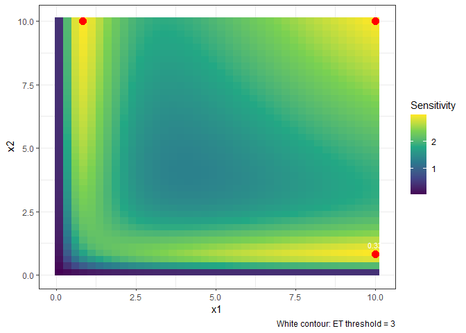

summary() gives additional detail: criterion value, Atwood convergence criterion, and the design space.

Other criteria

The same interface supports five optimality criteria:

Criterion	Key argument	Objective
`"D-Optimality"`	—	Minimise $-\log\det M$
`"Ds-Optimality"`	`par_int`	Focus on a subset of parameters
`"A-Optimality"`	—	Minimise $\operatorname{tr} M^{-1}$
`"I-Optimality"`	`reg_int`	Minimise integrated prediction variance
`"L-Optimality"`	`matB`	Minimise $\operatorname{tr}(B\,M^{-1})$

For example, A-Optimality minimises the average variance of all estimators:

result_A <- opt_des(
  criterion    = "A-Optimality",
  model        = y ~ Vmax * x1 * x2 / ((K1 + x1) * (K2 + x2)),
  parameters   = c("Vmax", "K1", "K2"),
  par_values   = c(1, 1, 1),
  design_space = list(x1 = c(0.1, 10), x2 = c(0.1, 10))
)
#> 
#> ℹ Stop condition not reached, max iterations performed
#> ⠙ Calculating optimal design 22 done (14/s) | 1.6sℹ The lower bound for efficiency is 99.9999976902864%
#>                                                    
result_A
#> Optimal design for A-Optimality (2 factors):
#>           x1         x2    Weight
#> 1  0.6569581 10.0000000 0.3725354
#> 2 10.0000000  0.6569844 0.3725333
#> 3 10.0000000 10.0000000 0.2549313

Compound criterion

Combine any set of criteria as a weighted sum. Weights are normalised automatically.

result_DI <- opt_des(
  criterion    = "Compound",
  model        = y ~ Vmax * x1 * x2 / ((K1 + x1) * (K2 + x2)),
  parameters   = c("Vmax", "K1", "K2"),
  par_values   = c(1, 1, 1),
  design_space = list(x1 = c(0.1, 10), x2 = c(0.1, 10)),
  compound     = list(
    list(criterion = "D-Optimality", weight = 0.6),
    list(criterion = "I-Optimality", weight = 0.4,
         reg_int = list(x1 = c(1, 5), x2 = c(1, 5)))
  )
)
#> ⠙ Calculating optimal design 7 done (3.3/s) | 2.1s⠹ Calculating optimal design 8 done (3.2/s) | 2.5s⠸ Calculating optimal design 9 done (3.1/s) | 2.9s⠼ Calculating optimal design 10 done (3/s) | 3.3s ⠴ Calculating optimal design 11 done (3.1/s) | 3.5s⠦ Calculating optimal design 13 done (3.4/s) | 3.8s⠧ Calculating optimal design 14 done (3.4/s) | 4.1s⠇ Calculating optimal design 16 done (3.6/s) | 4.4s⠏ Calculating optimal design 17 done (3.7/s) | 4.6s⠋ Calculating optimal design 18 done (3.8/s) | 4.8s⠙ Calculating optimal design 20 done (3.9/s) | 5.1s⠹ Calculating optimal design 21 done (4/s) | 5.3s  
#> ℹ Stop condition not reached, max iterations performed
#> ⠸ Calculating optimal design 22 done (4/s) | 5.5sℹ The lower bound for efficiency is 98.0491819762597%
#>                                                   
result_DI
#> Optimal design for Compound (0.60*D + 0.40*I):
#>           x1        x2    Weight
#> 1  0.9122428  8.703202 0.3548138
#> 2  1.6738998  1.439094 0.1073170
#> 3 10.0000000  1.012563 0.3389087
#> 4 10.0000000 10.000000 0.1989605

Design efficiency

design_efficiency() measures the fraction of the optimal information that a given design achieves. An efficiency of 0.80 means the design needs $1/0.80 = 1.25\times$ more observations to match the optimal.

corners <- data.frame(
  x1     = c(0.1, 10,  0.1, 10),
  x2     = c(0.1, 0.1, 10,  10),
  Weight = rep(0.25, 4)
)
eff <- design_efficiency(corners, result_D)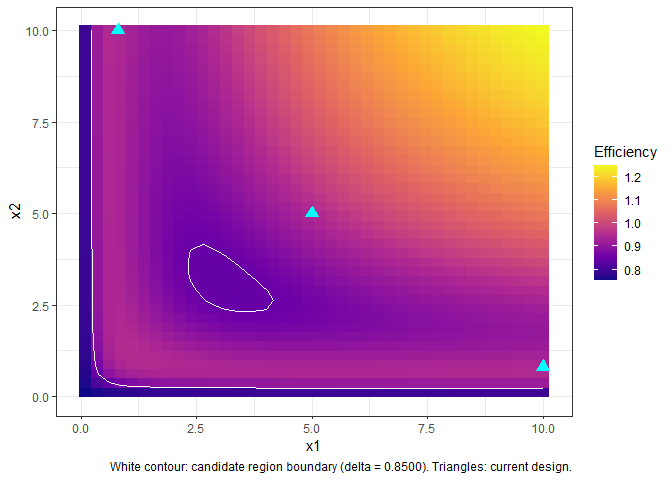
#> ℹ The efficiency of the design is 19.3350596170462%

Augmenting designs

get_augment_region() finds which points can be added to an existing design while keeping its D-efficiency above a threshold delta_val. augment_design() then adds the chosen point and rescales weights. Both functions work in 1D and multi-dimensional spaces.

init_des <- data.frame(
  x1     = c(0.8, 10,  5),
  x2     = c(10,  0.8, 5),
  Weight = c(1/3, 1/3, 1/3)
)

region <- get_augment_region(
  criterion           = "D-Optimality",
  init_design         = init_des,
  alpha               = 0.25,
  model               = y ~ Vmax * x1 * x2 / ((K1 + x1) * (K2 + x2)),
  parameters          = c("Vmax", "K1", "K2"),
  par_values          = c(1, 1, 1),
  design_space        = list(x1 = c(0.1, 10), x2 = c(0.1, 10)),
  calc_optimal_design = FALSE,
  delta_val           = 0.85
)

region$region contains the candidate points ranked by efficiency gain. Pick the best and augment:

best <- region$region[which.max(region$region$efficiency), ]

augmented <- augment_design(
  criterion           = "D-Optimality",
  init_design         = init_des,
  alpha               = 0.25,
  model               = y ~ Vmax * x1 * x2 / ((K1 + x1) * (K2 + x2)),
  parameters          = c("Vmax", "K1", "K2"),
  par_values          = c(1, 1, 1),
  design_space        = list(x1 = c(0.1, 10), x2 = c(0.1, 10)),
  calc_optimal_design = FALSE,
  delta_val           = 0.85,
  new_points          = data.frame(x1 = best$x1, x2 = best$x2, Weight = 1)
)

#> ℹ 1903 candidate points with efficiency >= 0.85 (from LHS sample of 2000)
#> Sample of candidate points:
#>           x1        x2 efficiency
#> 1  6.7385595 0.2924680  0.8909334
#> 2  1.9821626 1.1154958  0.9394470
#> 3  4.0971554 8.4766962  1.0007669
#> 4  6.0239305 8.7571051  1.1028042
#> 5  4.6024281 0.4528793  0.9276096
#> 6  9.4770793 4.5600493  1.0465406
#> 7  0.9444112 2.8258679  0.9368173
#> 8  8.0232267 1.8904368  0.8922271
#> 9  3.1618572 4.4661287  0.8625847
#> 10 5.0458372 9.1524421  1.0662419
#> 11 7.0391033 7.7941107  1.1160897
#> 12 0.4494250 7.4074376  0.9311998
#> 13 1.5010313 3.8698458  0.8872015
#> 14 8.1851605 4.7172844  1.0284918
#> 15 3.2994805 9.4786392  0.9698640
augmented
#>          x1        x2 Weight
#> 1  0.800000 10.000000   0.25
#> 2 10.000000  0.800000   0.25
#> 3  5.000000  5.000000   0.25
#> 4  9.912547  9.954952   0.25

Rounding to exact designs

Approximate designs assign continuous weights. Two functions convert them to integer replication counts for a given total $n$:

# Multiplier method
efficient_round(result_D$optdes, n = 12)
#>           x1         x2 Weight
#> 1  0.8332604 10.0000000      4
#> 2 10.0000000  0.8332352      4
#> 3 10.0000000 10.0000000      4

# Exhaustive floor/ceiling search (optimal for small number of support points)
combinatorial_round(result_D, n = 12)
#>           x1         x2 Weight
#> 1  0.8332604 10.0000000      4
#> 2 10.0000000  0.8332352      4
#> 3 10.0000000 10.0000000      4

KL-Optimality

KL-Optimality finds the design that maximises the Kullback-Leibler divergence between a reference model and the most adversarial rival, for Normal, Poisson, Binomial and Gamma families.

result_kl <- opt_des(
  "KL-Optimality",
  model        = y ~ Vmax * x / (Km + x),
  parameters   = c("Vmax", "Km"),
  par_values   = c(2, 1),
  design_space = c(0.1, 5),
  rival_model  = y ~ a * x,
  rival_params = c("a"),
  rival_pars   = c(1),
  rival_lower  = c(0.2),
  rival_upper  = c(2.5),
  family       = "Normal",
  phi          = 1
)
#> 
#> ℹ Stop condition reached: difference between sensitivity and criterion < 1e-05
#> ⠙ Calculating optimal design 7 done (8.1/s) | 863msℹ The lower bound for efficiency is 99.9957589718079%
#>                                                     
result_kl
#> Optimal design for KL-Optimality:
#>      Point    Weight
#> 1 1.127578 0.8159831
#> 2 5.000000 0.1840169
plot(result_kl)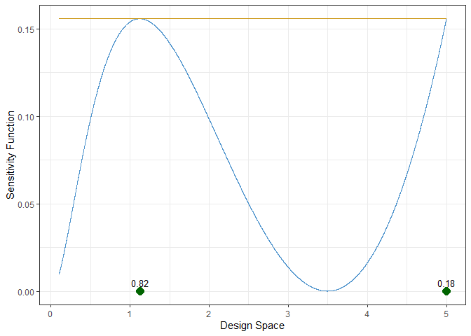

make_kl_fun() automates the KL function construction for custom model-family pairs, including different error structures or families.

Learn more

vignette("optedr-intro") — optimality criteria, multi-dimensional design spaces, compound designs, efficiency and rounding.
vignette("optedr-augment") — augmenting designs in 1D, 2D and 3D with controlled efficiency loss.
vignette("optedr-kl") — KL-Optimality for model discrimination, make_kl_fun(), and the Hill model case study.

Criterion	Key argument	Objective
`"D-Optimality"`	—	Minimise \(-\log\det M\)
`"Ds-Optimality"`	`par_int`	Focus on a subset of parameters
`"A-Optimality"`	—	Minimise \(\operatorname{tr} M^{-1}\)
`"I-Optimality"`	`reg_int`	Minimise integrated prediction variance
`"L-Optimality"`	`matB`	Minimise \(\operatorname{tr}(B\,M^{-1})\)