![]()
![]()
![]()
visOmopResults offers a set of functions tailored to
format objects of class <summarised_result> (as
defined in omopgenerics
package).
It provides functionalities to create formatted tables and generate plots. These visualisations are highly versatile for reporting results through Shiny apps, RMarkdown, Quarto, and more, supporting various output formats such as HTML, PNG, Word, and PDF.
You can install the latest version of visOmopResults from CRAN:
install.packages("visOmopResults")Or you can install the development version from GitHub with:
# install.packages("pak")
pak::pkg_install("darwin-eu/visOmopResults")
The <summarised_result> is a standardised output
format utilized across various packages, including:
Although this standard output format is essential, it can sometimes be challenging to manage. The visOmopResults package aims to simplify this process. To demonstrate the package’s functionality, let’s start by using some mock results:
library(visOmopResults)
result <- mockSummarisedResult()Currently all table functionalities are built around 4 packages: tibble, gt, flextable, and datatable.
There are two main functions:
visOmopTable(): Creates a well-formatted table
specifically from a <summarised_result> object.visTable(): Creates a nicely formatted table from any
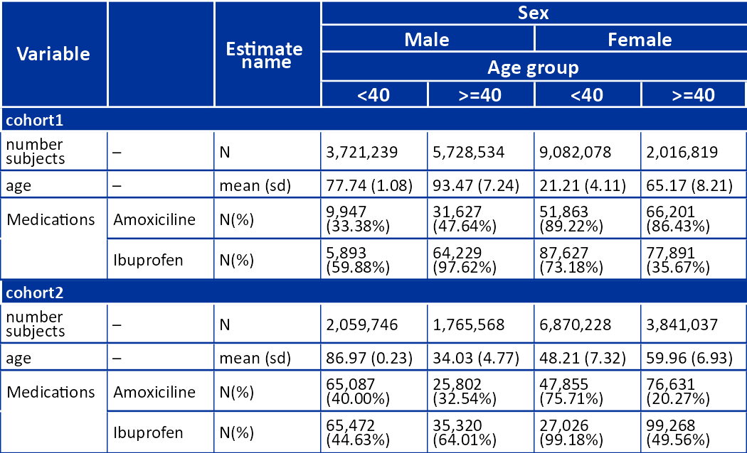
<data.frame> object.Let’s see a simple example:
result |>
  filterStrata(sex != "overall" & age_group != "overall") |>
  visOmopTable(
    type = "flextable",
    estimateName = c(
      "N(%)" = "<count> (<percentage>%)",
      "N" = "<count>",
      "mean (sd)" = "<mean> (<sd>)"),
    header = c("sex", "age_group"),
    settingsColumn = NULL,
    groupColumn = c("cohort_name"),
    rename = c("Variable" = "variable_name", " " = "variable_level"),
    hide = "cdm_name",
    style = "darwin"
  )
Currently all plot functionalities are built around ggplot2. The
output of these plot functions is a <ggplot2> object
that can be further customised.
There are three plotting functions:
plotScatter() to create a scatter plot.plotBar() to create a bar plot.plotBox() to create a box plot.Additionally, the themeVisOmop() function applies a
consistent styling to the plots, aligning them with the package’s visual
design.
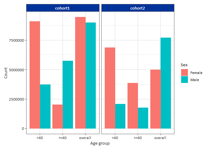
Let’s see how we can create a simple boxplot for age:
library(dplyr)
result |>
  filter(variable_name == "number subjects") |>
  filterStrata(sex != "overall") |>
  barPlot(
    x = "age_group",
    y = "count",
    facet = "cohort_name",
    colour = "sex",
    style = "darwin"
  )